General Case of the Wigner Rotation
Table of Contents
The Wigner rotation states that the successive application of two Lorentz boosts in arbitrary directions to a reference frame is equivalent to a single Lorentz boost together with a spatial rotation.
Namely
$$ \hat{Q}\left(\boldsymbol{\beta}_{2}\right) \hat{Q}\left(\boldsymbol{\beta}_{1}\right) = \hat{Q}\left(\boldsymbol{\beta} \right) \hat{R} \tag{1} $$This article aims to treat the general case of the Wigner rotation.
Vector Form of the Relativistic Transformation #
We first derive the matrix form of an arbitrary Lorentz boost in vector notation. Let \(\boldsymbol{\beta}\) characterize the Lorentz boost. For an event with coordinates \(( \boldsymbol{x},\ x^{0} = ct)\) in frame \(S\), the spatial vector \(\boldsymbol{x}\) can be decomposed into components parallel and perpendicular to the boost direction
$$ \begin{align} \boldsymbol{x} & = x_{\parallel } \boldsymbol{e_{\parallel}} + x_{\bot} \boldsymbol{e_{\bot}} \notag \\ & = \boldsymbol{x} \cdot \frac{\boldsymbol{\beta}}{\beta} \frac{\boldsymbol{\beta}}{\beta} + \left( \boldsymbol{x} - \boldsymbol{x} \cdot \frac{\boldsymbol{\beta}}{\beta} \frac{\boldsymbol{\beta}}{\beta} \right) \tag{2} \end{align} $$Using the Lorentz transformation formulas we obtain
$$ \begin{align} \boldsymbol{x'} & = \gamma \left( \boldsymbol{x} \cdot \frac{\boldsymbol{\beta}}{\beta} - \beta x^0 \right) \frac{\boldsymbol{\beta}}{\beta} + \left( \boldsymbol{x} - \boldsymbol{x} \cdot \frac{\boldsymbol{\beta}}{\beta} \frac{\boldsymbol{\beta}}{\beta} \right) \notag \\ & = \left[ \mathbf{I} + (\gamma - 1) \frac{\boldsymbol{\beta}}{\beta} \frac{\boldsymbol{\beta}}{\beta} \right] \cdot \boldsymbol{x} - \gamma \boldsymbol{\beta} x^0 \tag{3a} \\ x'^0 & = \gamma x^0 - \boldsymbol{\beta} \gamma \cdot \boldsymbol{x} \tag{3b} \end{align} $$This can be written in matrix form as
$$ \begin{bmatrix} \boldsymbol{x'} \\ x'^0 \end{bmatrix} = \begin{bmatrix} \mathbf{I} + (\gamma - 1) \frac{\boldsymbol{\beta}}{\beta} \frac{\boldsymbol{\beta}}{\beta} & -\boldsymbol{\beta} \gamma \\ -\boldsymbol{\beta} \gamma & \gamma \end{bmatrix} \begin{bmatrix} \boldsymbol{x} \\ x^0 \end{bmatrix} \tag{4} $$Let \(\gamma = \ch \theta\), then \(\beta \gamma = \sh \theta\).
Let \(\frac{\boldsymbol{\beta}}{\beta} = \boldsymbol{e}\) be the unit vector along the boost direction. Then
$$ \hat{Q}(\boldsymbol{\beta}) = \begin{bmatrix} \mathbf{I} + (\ch \theta - 1) \boldsymbol{e} \boldsymbol{e} & -\sh \theta \boldsymbol{e} \\ -\sh \theta \boldsymbol{e} & \ch \theta \end{bmatrix} \tag{5} $$Determining the Equivalent Lorentz Boost \(\boldsymbol{\beta}\) #
For two successive Lorentz boosts in arbitrary directions we write
$$ \begin{align} & \hat{Q}\left(\boldsymbol{\beta}_{2}\right) \hat{Q}\left(\boldsymbol{\beta}_{1}\right) \notag \\ & = \begin{bmatrix} \mathbf{I} + (\ch \theta_2 - 1) \boldsymbol{e}_2 \boldsymbol{e}_2 & -\sh \theta_2 \boldsymbol{e}_2 \\ -\sh \theta_2 \boldsymbol{e}_2 & \ch \theta_2 \end{bmatrix} \begin{bmatrix} \mathbf{I} + (\ch \theta_1 - 1) \boldsymbol{e}_1 \boldsymbol{e}_1 & -\sh \theta_1 \boldsymbol{e}_1 \\ -\sh \theta_1 \boldsymbol{e}_1 & \ch \theta_1 \end{bmatrix} \notag \\ & = \begin{bmatrix} \mathbf{A}_{11} & \boldsymbol{a}_{12} \\ \boldsymbol{a}_{21} & a_{22} \end{bmatrix} \tag{6} \end{align} $$where
$$ \begin{align} \mathbf{A}_{11} & = \mathbf{I} + (\ch\theta_1 - 1)\boldsymbol{e}_1\boldsymbol{e}_1 + (\ch\theta_2 - 1)\boldsymbol{e}_2\boldsymbol{e}_2 + \left[(\ch\theta_1 - 1)(\ch\theta_2 - 1)\boldsymbol{e}_1 \cdot \boldsymbol{e}_2 + \sh\theta_1\sh\theta_2 \right]\boldsymbol{e}_2 \boldsymbol{e}_1 \notag \quad \text{(7a)} \\ \boldsymbol{a}_{12} & = -\sh\theta_1\boldsymbol{e}_1 - \left[\sh\theta_1(\ch\theta_2 - 1)\boldsymbol{e}_1\cdot \boldsymbol{e}_2 + \sh\theta_2\ch\theta_1\right]\boldsymbol{e}_2 \tag{7b} \\ \boldsymbol{a}_{21} & = -\sh\theta_2\boldsymbol{e}_2 - \left[\sh\theta_2(\ch\theta_1 - 1)\boldsymbol{e}_1\cdot \boldsymbol{e}_2 + \ch\theta_2\sh\theta_1\right]\boldsymbol{e}_1 \tag{7c} \\ a_{22} & = \sh\theta_1\sh\theta_2\boldsymbol{e}_1\cdot \boldsymbol{e}_2 + \ch\theta_1\ch\theta_2 \tag{7d} \end{align} $$We first look ahead at the relation to be established
$$ \hat{Q}\left(\boldsymbol{\beta}_{2}\right) \hat{Q}\left(\boldsymbol{\beta}_{1}\right) = \hat{Q}\left(\boldsymbol{\beta} \right) \hat{R} \tag{8} $$For the left-hand side
$$ \hat{Q}\left(\boldsymbol{\beta}_{2}\right) \hat{Q}\left(\boldsymbol{\beta}_{1}\right) = \begin{bmatrix} \mathbf{A}_{11} & \boldsymbol{a}_{12} \\ \boldsymbol{a}_{21} & a_{22} \end{bmatrix} \tag{9} $$For the right-hand side
$$ \begin{align} \hat{Q}\left(\boldsymbol{\beta} \right) \hat{R} & = \begin{bmatrix} \mathbf{I} + (\ch\theta - 1)\boldsymbol{e}\boldsymbol{e} & -\sh\theta\boldsymbol{e} \\ -\sh\theta\boldsymbol{e} & \ch\theta \end{bmatrix} \begin{bmatrix} \mathbf{R}_{11} & 0 \\ 0 & 1 \end{bmatrix} \notag \\ & = \begin{bmatrix} (\mathbf{I} + (\ch\theta - 1)\boldsymbol{e}\boldsymbol{e})\cdot \mathbf{R}_{11} & -\sh\theta\boldsymbol{e} \\ -\sh\theta\boldsymbol{e}\cdot \mathbf{R}_{11} & \ch\theta \end{bmatrix} \tag{10} \end{align} $$Note that here (and below) \(\boldsymbol{e} \cdot \mathbf{R}_{11}\) denotes \(e_i R_{ij}\), i.e. \(\boldsymbol{e}^T \mathbf{R}_{11}\).
Moreover, \(\mathbf{R}_{11}\) is a (pure) rotation matrix.
Thus to verify equality of the two sides we proceed:
- Verify \(a_{22}^2 - |\boldsymbol{a}_{12}|^2 = 1\), which allows extraction of \n> \(\boldsymbol{\beta}\).
- Make an ansatz for \(\boldsymbol{\beta}\).
- Using the ansatz compute \(\hat{R} = \hat{Q}^{-1}(\boldsymbol{\beta})\hat{Q}(\boldsymbol{\beta_2})\hat{Q}(\boldsymbol{\beta_1})\).
- Show \(\hat{R}\) is a pure spatial rotation; the ansatz is then confirmed.
We can verify
$$ \begin{cases} a_{22}^2 - |\boldsymbol{a}_{12}|^2 = 1 \\ a_{22}^2 - |\boldsymbol{a}_{21}|^2 = 1 \tag{11} \end{cases} $$Hence define
$$ \begin{align} \ch\theta &= a_{22} = \sh\theta_1\sh\theta_2\boldsymbol{e}_1\cdot\boldsymbol{e}_2 + \ch\theta_1\ch\theta_2 \tag{12a} \\ \sh\theta &= |\boldsymbol{a}_{12}| = |\boldsymbol{a}_{21}| \tag{12b} \end{align} $$For the direction \(\boldsymbol{e}\) of \(\boldsymbol{\beta}\) we posit
$$ -\sh\theta\ \ \boldsymbol{e} = \boldsymbol{a}_{12} \tag{13} $$which gives
$$ \boldsymbol{e} = \frac{\sh\theta_1\boldsymbol{e}_1 + \left[\sh\theta_1(\ch\theta_2 - 1)\boldsymbol{e}_1\cdot \boldsymbol{e}_2 + \sh\theta_2\ch\theta_1\right]\boldsymbol{e}_2}{\sqrt{\sh^2\theta_1 \sh^2\theta_2(\boldsymbol{e}_1\cdot \boldsymbol{e}_2)^2 + \ch^2\theta_1\ch^2\theta_2 + 2\sh\theta_1\sh\theta_2\ch\theta_1\ch\theta_2(\boldsymbol{e}_1\cdot \boldsymbol{e}_2) - 1}} \quad \text{(14)} $$Therefore
$$ \hat{Q}(\boldsymbol{\beta}) = \begin{bmatrix} \mathbf{I} + (\ch\theta - 1)\boldsymbol{e}\boldsymbol{e} & -\sh\theta\boldsymbol{e} \\ -\sh\theta\boldsymbol{e} & \ch\theta \end{bmatrix} \tag{15} $$Verifying the Spatial Rotation \(\hat{R}\) #
$$ \begin{align} \hat{R} & = \hat{Q}^{-1}(\boldsymbol{\beta})\hat{Q}(\boldsymbol{\beta_2})\hat{Q}(\boldsymbol{\beta_1}) \notag \\ & = \hat{Q}(-\boldsymbol{\beta})\hat{Q}(\boldsymbol{\beta_2})\hat{Q}(\boldsymbol{\beta_1}) \notag \\ & = \begin{bmatrix} 1 + (\ch\theta - 1)\boldsymbol{e}\boldsymbol{e} & \sh\theta\boldsymbol{e} \\ \sh\theta\boldsymbol{e} & \ch\theta \end{bmatrix} \begin{bmatrix} \mathbf{A}_{11} & \boldsymbol{a}_{12} \\ \boldsymbol{a}_{21} & a_{22} \end{bmatrix} \notag \\ & = \begin{bmatrix} \mathbf{R}_{11} & \boldsymbol{r}_{12} \\ \boldsymbol{r}_{21} & r_{22} \end{bmatrix} \tag{16} \end{align} $$with
$$ \begin{align} r_{22} & = \sh\theta\boldsymbol{e}\cdot\boldsymbol{a}_{12} + \ch\theta \ a_{22} \notag \\ & = \sh\theta\boldsymbol{e} \cdot (-\sh\theta\boldsymbol{e}) + \ch^2\theta \notag \\ & = -\sh^2\theta|\boldsymbol{e}|^2 + \ch^2\theta = 1 \tag{17a} \\ \boldsymbol{r}_{12} & = \left[ \mathbf{I} + (\ch\theta - 1)\boldsymbol{e}\boldsymbol{e} \right] \cdot \boldsymbol{a}_{12} + \sh\theta \boldsymbol{e}\ a_{22} \notag \\ & = \left[ \mathbf{I} + (\ch\theta - 1)\boldsymbol{e}\boldsymbol{e} \right] \cdot (-\sh\theta \boldsymbol{e}) + \sh\theta \ch\theta \boldsymbol{e} \notag \\ & = \boldsymbol{0} \tag{17b} \\ \boldsymbol{r}_{21} & = \sh\theta \boldsymbol{e} \cdot \mathbf{A}_{11} + \ch\theta \boldsymbol{a}_{21} \notag \\ & = -\boldsymbol{a}_{12} \cdot \mathbf{A}_{11} + a_{22} \boldsymbol{a}_{21} \notag \\ & = \boldsymbol{0} \tag{17c} \\ \mathbf{R}_{11} & = \left[ \mathbf{I} + (\ch\theta - 1)\boldsymbol{e}\boldsymbol{e} \right] \cdot \mathbf{A}_{11} + \sh\theta \boldsymbol{e} \boldsymbol{a}_{21} \tag{17d} \\ \end{align} $$We observe that \(r_{22} = 1\) and \(\boldsymbol{r}_{12}=\boldsymbol{0}\); thus indeed \(-\sh\theta\ \ \boldsymbol{e} = \boldsymbol{a}_{12}\), confirming the ansatz (13).
Next we must show that \(\mathbf{R}_{11}\) is a pure rotation matrix.
Since
$$ \boldsymbol{r}_{21} = \sh\theta \boldsymbol{e} \cdot \mathbf{A}_{11} + \ch\theta \boldsymbol{a}_{21} = \boldsymbol{0} \tag{18} $$we have
$$ \begin{align} \mathbf{R}_{11} & = \left[ \mathbf{I} + (\ch\theta - 1)\boldsymbol{e}\boldsymbol{e} \right] \cdot \mathbf{A}_{11} + \sh\theta \boldsymbol{e} \frac{ - \sh\theta\boldsymbol{e} \cdot \mathbf{A}_{11}}{\ch\theta} \notag \\ & = \left[ \mathbf{I} - \frac{\ch\theta - 1}{\ch\theta} \boldsymbol{e}\boldsymbol{e} \right] \cdot \mathbf{A}_{11} \notag \\ & = \left[ \mathbf{I} - \frac{1}{\ch\theta (\ch\theta + 1)} \boldsymbol{a}_{12} \boldsymbol{a}_{12} \right] \cdot \mathbf{A}_{11} \notag \\ & = \mathbf{I} + b_{11} \boldsymbol{e}_1 \boldsymbol{e}_1 + b_{12} \boldsymbol{e}_1 \boldsymbol{e}_2 + b_{21} \boldsymbol{e}_2 \boldsymbol{e}_1 + b_{22} \boldsymbol{e}_2 \boldsymbol{e}_2 \tag{19} \end{align} $$We have written \(\mathbf{R}_{11}\) in the form (19), i.e.
$$ \begin{align} \mathbf{R}_{11} & = \mathbf{I} + \sum b_{ij} \boldsymbol{e}_i \boldsymbol{e}_j \notag \\ & = \mathbf{I} + \begin{bmatrix} \boldsymbol{e}_1 & \boldsymbol{e}_2 \end{bmatrix} \begin{bmatrix} b_{11} & b_{12} \\ b_{21} & b_{22} \end{bmatrix} \begin{bmatrix} \boldsymbol{e}_1 \\ \boldsymbol{e}_2 \end{bmatrix} \tag{20} \end{align} $$To show it is a rotation matrix we must verify
$$ \mathbf{R}_{11} \mathbf{R}_{11}^T = \mathbf{I} \tag{21} $$$$ \det \mathbf{R}_{11} = 1 \tag{22} $$
Using (20), equation (21) can be simplified as
$$ \begin{bmatrix} b_{11} & b_{12} \\ b_{21} & b_{22} \end{bmatrix} + \begin{bmatrix} b_{11} & b_{21} \\ b_{12} & b_{22} \end{bmatrix} + \begin{bmatrix} b_{11} & b_{12} \\ b_{21} & b_{22} \end{bmatrix} \begin{bmatrix} 1 & \boldsymbol{e}_1 \cdot \boldsymbol{e}_2 \\ \boldsymbol{e}_1 \cdot \boldsymbol{e}_2 & 1 \end{bmatrix} \begin{bmatrix} b_{11} & b_{21} \\ b_{12} & b_{22} \end{bmatrix} = 0 \tag{23} $$For (22), multiplying (20) on the right by \(\begin{bmatrix} \boldsymbol{e}_1 & \boldsymbol{e}_2 \end{bmatrix}\) gives
$$ \mathbf{R}_{11} \begin{bmatrix} \boldsymbol{e}_1 & \boldsymbol{e}_2 \end{bmatrix} = \begin{bmatrix} \boldsymbol{e}_1 & \boldsymbol{e}_2 \end{bmatrix} \left( \mathbf{I} + \begin{bmatrix} b_{11} & b_{12} \\ b_{21} & b_{22} \end{bmatrix} \begin{bmatrix} 1 & \boldsymbol{e}_1 \cdot \boldsymbol{e}_2 \\ \boldsymbol{e}_1 \cdot \boldsymbol{e}_2 & 1 \end{bmatrix} \tag{24} \right) $$Since
$$ \det \begin{bmatrix} \boldsymbol{e}_1 & \boldsymbol{e}_2 \end{bmatrix} = \sqrt{1 - (\boldsymbol{e}_1 \cdot \boldsymbol{e}_2)^2} \neq 0 \tag{25} $$we obtain
$$ \det \mathbf{R}_{11} = \det \left( \mathbf{I} + \begin{bmatrix} b_{11} & b_{12} \\ b_{21} & b_{22} \end{bmatrix} \begin{bmatrix} 1 & \boldsymbol{e}_1 \cdot \boldsymbol{e}_2 \\ \boldsymbol{e}_1 \cdot \boldsymbol{e}_2 & 1 \end{bmatrix} \right) = 1 \tag{26} $$Thus, we need to verify (23) and (26).
The coefficients are
$$ \begin{align} & b_{11} = b_{22} = - \frac{(\ch\theta_1 - 1)(\ch\theta_2 - 1)}{\ch\theta + 1} \tag{27a} \\ & b_{12} = -\frac{\sh\theta_1 \sh\theta_2}{\ch\theta + 1} \tag{27b} \\ & b_{21} = \frac{2(\ch\theta_1 - 1)(\ch\theta_2 - 1)(\boldsymbol{e}_1 \cdot \boldsymbol{e}_2) + \sh\theta_1 \sh\theta_2}{\ch\theta + 1} \tag{27c} \\ \end{align} $$They satisfy
$$ \begin{cases} b_{11} = b_{22}\\ (b_{11}+1)(b_{22}+1) - b_{12}b_{21} = 1 \\ b_{12} + b_{21} + 2b_{22}(\boldsymbol{e}_1 \cdot \boldsymbol{e}_2) = 0 \end{cases} \tag{28} $$Hence \(\mathbf{R}_{11}\) is a rotation matrix.
Therefore
$$ \hat{R}= \begin{bmatrix} \mathbf{R}_{11} & 0 \\ 0 & 1 \end{bmatrix} \tag{29} $$corresponding to a spatial rotation.
Vector Form of the Rotation Matrix \(\mathbf{R}_{11}\) #
We first recall the matrix representation of an arbitrary rotation to guide simplification and analysis.
Any rotation can be described by a unit rotation axis \(\boldsymbol{n}\) and rotation angle \(\phi\).
As shown in the figure
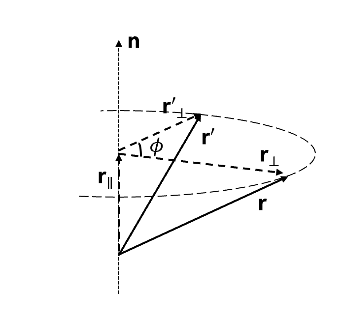
Figure 1 We have
$$ \boldsymbol{r}' = \boldsymbol{r}_\parallel + \boldsymbol{r}'_\bot \tag{30}$$where
$$ \boldsymbol{r}_\parallel = (\boldsymbol{r} \cdot \boldsymbol{n}) \boldsymbol{n} \tag{31} $$$$ \boldsymbol{r}'_\bot = \boldsymbol{r}_\bot \cos\phi + (\boldsymbol{n} \times \boldsymbol{r}_\bot) \sin\phi \tag{32} $$
Thus
$$ \boldsymbol{r}' = (\boldsymbol{r} \cdot \boldsymbol{n}) \boldsymbol{n} + (\boldsymbol{r} - (\boldsymbol{r} \cdot \boldsymbol{n}) \boldsymbol{n}) \cos\phi + (\boldsymbol{n} \times \boldsymbol{r}) \sin\phi \tag{33} $$i.e.
$$ r'_i = \left[ n_i n_j + (\delta_{ij} - n_i n_j) \cos\phi - \varepsilon_{ijk} n_k \sin\phi \right] r_j \tag{34} $$yielding the rotation matrix
$$ R_{ij} = n_i n_j + (\delta_{ij} - n_i n_j) \cos\phi - \varepsilon_{ijk} n_k \sin\phi \tag{35} $$
We now decompose the identity \(\mathbf{I}\).
Our goal is to decompose the identity appearing in (19). The ambient space is \(\mathbb{R}^3\); hence \( (\operatorname{span}\{\boldsymbol{e}_1, \boldsymbol{e}_2\})^\perp \cong \mathbb{R}^1\). Let \(\boldsymbol{e}_{\bot}\) be a unit vector spanning this orthogonal complement.
Let
$$ \mathbf{I} = C_{11} \boldsymbol{e}_1\boldsymbol{e}_1 + C_{12} \boldsymbol{e}_1\boldsymbol{e}_2 + C_{21} \boldsymbol{e}_2\boldsymbol{e}_1 + C_{22} \boldsymbol{e}_2\boldsymbol{e}_2 + \boldsymbol{e}_{\bot} \boldsymbol{e}_{\bot} \tag{36} $$Then
$$ C_{11} = C_{22} = \frac{1}{1 - (\boldsymbol{e}_1 \cdot \boldsymbol{e}_2)^2} \tag{37} $$$$ C_{12} = C_{21} = -\frac{\boldsymbol{e}_1 \cdot \boldsymbol{e}_2}{1 - (\boldsymbol{e}_1 \cdot \boldsymbol{e}_2)^2} \tag{38} $$
Thus
$$ \begin{align} \mathbf{R}_{11} &= \left( 1 + \frac{b_{11}}{C_{11}} \right) \mathbf{I} - \frac{b_{11}}{C_{11}} \mathbf{I} + b_{11} \boldsymbol{e}_1 \boldsymbol{e}_1 + b_{12} \boldsymbol{e}_1 \boldsymbol{e}_2 + b_{21} \boldsymbol{e}_2 \boldsymbol{e}_1 + b_{22} \boldsymbol{e}_2 \boldsymbol{e}_2 \notag \\ &= \left( 1 + \frac{b_{11}}{C_{11}} \right) \mathbf{I} + \left( b_{11} - b_{11}\frac{C_{11}}{C_{11}} \right) \boldsymbol{e}_1\boldsymbol{e}_1 + \left( b_{12} - b_{11}\frac{C_{12}}{C_{11}} \right) \boldsymbol{e}_1\boldsymbol{e}_2 \notag \\ &\phantom{{}= \left( 1 + \frac{b_{11}}{C_{11}} \right) \mathbf{I}} + \left( b_{21} - b_{11}\frac{C_{21}}{C_{11}} \right) \boldsymbol{e}_2\boldsymbol{e}_1 + \left( b_{22} - b_{11}\frac{C_{22}}{C_{11}} \right) \boldsymbol{e}_2\boldsymbol{e}_2 \notag \\ &\phantom{{}= \left( 1 + \frac{b_{11}}{C_{11}} \right) \mathbf{I}} - \frac{b_{11}}{C_{11}} \boldsymbol{e}_{\bot} \boldsymbol{e}_{\bot} \notag \\ &= \boldsymbol{e}_{\bot} \boldsymbol{e}_{\bot} + \left( \mathbf{I} -\boldsymbol{e}_{\bot} \boldsymbol{e}_{\bot} \right) \left( 1 + \frac{b_{11}}{C_{11}} \right) + \left( b_{12} - b_{11}\frac{C_{12}}{C_{11}} \right) \boldsymbol{e}_1\boldsymbol{e}_2 \notag \\ &\phantom{= \boldsymbol{e}_{\bot} \boldsymbol{e}_{\bot} + \left( \mathbf{I} -\boldsymbol{e}_{\bot} \boldsymbol{e}_{\bot} \right) \left( 1 + \frac{b_{11}}{C_{11}} \right)} + \left( b_{21} - b_{11}\frac{C_{21}}{C_{11}} \right) \boldsymbol{e}_2\boldsymbol{e}_1 \notag \\ &= \boldsymbol{e}_{\bot} \boldsymbol{e}_{\bot} + \left( \mathbf{I} -\boldsymbol{e}_{\bot} \boldsymbol{e}_{\bot} \right) \left[ \alpha (\boldsymbol{e}_1 \cdot \boldsymbol{e}_2) + \beta \right] + \alpha \left[ \boldsymbol{e}_2\boldsymbol{e}_1 - \boldsymbol{e}_1\boldsymbol{e}_2 \right] \tag{39} \end{align} $$Or
$$ (\mathbf{R}_{11})_{ij} = (\boldsymbol{e}_{\bot})_i (\boldsymbol{e}_{\bot})_j + \left[ \delta_{ij} - (\boldsymbol{e}_{\bot})_i (\boldsymbol{e}_{\bot})_j \right] \left[ \alpha (\boldsymbol{e}_1 \cdot \boldsymbol{e}_2) + \beta \right] - \alpha \varepsilon_{ijk} (\boldsymbol{e}_1 \times \boldsymbol{e}_2)_k \quad \text{(40)} $$with
$$ \begin{cases} \alpha = \frac{\sh\theta_1\sh\theta_2 + (\ch\theta_1-1)(\ch\theta_2-1)(\boldsymbol{e_1} \cdot \boldsymbol{e_2})}{\ch\theta+1} \\ \beta = \frac{\ch\theta_1+\ch\theta_2}{\ch\theta+1} \end{cases} \tag{41} $$Denote the rotation angle by \(\phi\) and its axis by \(\boldsymbol{n}\). Comparing with (35) we identify
$$ \begin{aligned} \boldsymbol{n} \sin\phi & = \alpha (\boldsymbol{e}_1 \times \boldsymbol{e}_2) \notag \\ & = \frac{\sh\theta_1 \sh\theta_2 + (\ch\theta_1 - 1)(\ch\theta_2 - 1)(\boldsymbol{e}_1 \cdot \boldsymbol{e}_2)}{\ch\theta + 1} \boldsymbol{e}_1 \times \boldsymbol{e}_2 \notag \\ & = \frac{\sh\theta_1 \sh\theta_2 + (\ch\theta_1 - 1)(\ch\theta_2 - 1)(\boldsymbol{e}_1 \cdot \boldsymbol{e}_2)}{\sh\theta_1 \sh\theta_2 (\boldsymbol{e}_1 \cdot \boldsymbol{e}_2) + \ch\theta_1 \ch\theta_2 + 1} \boldsymbol{e}_1 \times \boldsymbol{e}_2 \quad \text{(42)} \end{aligned} $$Supplementary Material #
(i) Order of the Equivalent Boost and Rotation #
The equivalent transformation considered above is
$$ \hat{Q}\left(\boldsymbol{\beta}_{2}\right) \hat{Q}\left(\boldsymbol{\beta}_{1}\right) = \hat{Q}\left(\boldsymbol{\beta} \right) \hat{R} \tag{43} $$That is: rotation first, then the (net) Lorentz boost.
In fact there are two equivalent forms
$$ \hat{Q}\left(\boldsymbol{\beta}_{2}\right) \hat{Q}\left(\boldsymbol{\beta}_{1}\right) = \hat{Q}\left(\boldsymbol{\beta} \right) \hat{R} = \hat{R}' \hat{Q}\left(\boldsymbol{\beta}' \right) \tag{44} $$We compare the two. Interchanging the order changes the off-diagonal block elements
$$ \hat{Q}\left(\boldsymbol{\beta} \right) \hat{R} = \begin{bmatrix} (\mathbf{I} + (\ch\theta - 1)\boldsymbol{e}\boldsymbol{e})\cdot \mathbf{R}_{11} & -\sh\theta\boldsymbol{e} \\ -\sh\theta\boldsymbol{e}\cdot \mathbf{R}_{11} & \ch\theta \end{bmatrix} \tag{45} $$$$ \hat{R}' \hat{Q}\left(\boldsymbol{\beta}' \right) = \begin{bmatrix} \mathbf{R}'_{11} \cdot (\mathbf{I} + (\ch\theta' - 1)\boldsymbol{e}'\boldsymbol{e}') & -\sh\theta'\ \mathbf{R}'_{11} \cdot \boldsymbol{e}' \\ -\sh\theta'\ \boldsymbol{e}' & \ch\theta' \end{bmatrix} \tag{46} $$
We see that \(|\boldsymbol{\beta}'| = |\boldsymbol{\beta}|\) but the direction is rotated
$$ \begin{cases} \boldsymbol{\beta} = \mathbf{R}'_{11} \cdot \boldsymbol{\beta}'\\ \boldsymbol{\beta}' = \boldsymbol{\beta} \cdot \mathbf{R}_{11} \end{cases} \tag{47} $$or
$$ \begin{cases} \beta_i = R'_{ij} \beta'_j \\ \beta'_i = \beta_j R_{ji} \end{cases} \tag{48} $$Thus
$$ \beta_i = R'_{ij} \beta_k R_{kj} \tag{49}$$so that
$$ R'_{ij} R_{kj} = \delta_{ik} \tag{50}$$or
$$ \mathbf{R}'_{11} \mathbf{R}_{11}^T = \mathbf{I} \tag{51}$$which implies
$$ \mathbf{R}'_{11} = \mathbf{R}_{11} \tag{52}$$Therefore
$$ \hat{Q}\left(\boldsymbol{\beta}_{2}\right) \hat{Q}\left(\boldsymbol{\beta}_{1}\right) = \hat{Q}\left(\boldsymbol{\beta} \right) \hat{R} = \hat{R} \hat{Q}\left( \mathbf{R}_{11}^T \cdot \boldsymbol{\beta} \right) \tag{53} $$Alternatively,
$$\hat{Q}\left( \mathbf{R}_{11}^T \cdot \boldsymbol{\beta} \right) = \hat{R}^T \hat{Q}\left(\boldsymbol{\beta} \right) \hat{R} \tag{54}$$which is immediate from spatial rotational symmetry of the Lorentz group.
(ii) Low-Velocity Approximation #
Consider the limit \(\beta_1, \beta_2 \to 0\). Then
$$ \begin{align} \boldsymbol{n} \sin\phi & = \frac{\gamma_1 \gamma_2 \beta_1 \beta_2 + (\gamma_1 - 1)(\gamma_2 - 1)(\boldsymbol{e}_1 \cdot \boldsymbol{e}_2)}{\gamma_1 \gamma_2 \beta_1 \beta_2 (\boldsymbol{e}_1 \cdot \boldsymbol{e}_2) + \gamma_1 \gamma_2 + 1} \boldsymbol{e}_1 \times \boldsymbol{e}_2 \notag \\ & \approx \frac{1}{2} \beta_1 \beta_2 \boldsymbol{e}_1 \times \boldsymbol{e}_2 \notag \\ & = \frac{1}{2} \boldsymbol{\beta}_1 \times \boldsymbol{\beta}_2 \tag{55} \end{align} $$Thus \(\sin\phi \approx \phi\) and
$$ \boldsymbol{n} \phi = \frac{1}{2} \boldsymbol{\beta}_1 \times \boldsymbol{\beta}_2 \tag{56} $$(iii) Thomas Precession #
Thomas precession states that the proper frame of a particle moving along a curved trajectory (i.e. with acceleration having a component perpendicular to its velocity) undergoes a purely relativistic precession relative to the laboratory frame.
At times \(t\) and \(t+dt\) let the instantaneous rest frames be \(S\) and \(S'\), respectively. The transformation between them can be expressed as the composition of two boosts
$$ S \to S' :\quad \hat{\Lambda} = \hat{Q}\!\left(\boldsymbol{\beta}+d\boldsymbol{\beta}\right)\hat{Q}\!\left(\boldsymbol{- \beta}\right) \tag{57} $$Here \(\hat{Q}\!\left(\boldsymbol{- \beta}\right)\) takes \(S\) back to the lab frame, then \(\hat{Q}\!\left(\boldsymbol{\beta}+d\boldsymbol{\beta}\right)\) carries the lab to the new instantaneous rest frame \(S'\). With
$$\boldsymbol{\beta} = \frac{\boldsymbol{v}}{c}, \quad d\boldsymbol{\beta} = \frac{\boldsymbol{a} dt}{c} \tag{58}$$Using (42) and \(d\boldsymbol{\beta} \ll \boldsymbol{\beta}\), keeping first order
$$ \boldsymbol{n} \sin d\phi \approx \frac{\gamma^2 \beta^2 - (\gamma - 1)^2}{ - \gamma^2 \beta^2 + \gamma^2 + 1} \frac{ - \boldsymbol{\beta} \times d\boldsymbol{\beta}}{\beta^2} = \frac{ 1- \gamma }{\beta^2} \boldsymbol{\beta} \times d\boldsymbol{\beta} = \frac{\gamma^2}{\gamma + 1} d\boldsymbol{\beta} \times \boldsymbol{\beta} \tag{59} $$Thus
$$\boldsymbol{n} d{\phi} = \frac{\gamma^2}{\gamma + 1} d\boldsymbol{\beta} \times \boldsymbol{\beta} = \frac{\gamma^2}{\gamma + 1} \frac{dt}{c^2} \boldsymbol{a} \times \boldsymbol{v} \tag{60}$$The Thomas precession angular velocity is
$$ \boldsymbol{\omega}_T = \frac{\gamma^2}{\gamma + 1} \frac{ \boldsymbol{a} \times \boldsymbol{v} }{c^2} \tag{61} $$For \(v \ll c\)
$$ \boldsymbol{\omega}_T \approx \frac{1}{2} \frac{ \boldsymbol{a} \times \boldsymbol{v} }{c^2} \tag{62} $$In the Bohr model of hydrogen this yields
$$ \omega_T = \frac{\mu_0}{8\pi} \frac{m e^8}{(4\pi \epsilon_0)^3 (n \hbar)^5} \tag{63} $$(iv) Algebraic Structure #
The Wigner rotation originates from the non-vanishing commutator of the Lorentz boost generators \(\hat{\boldsymbol{K}}\).
Let the rapidities of the two boosts be \(\boldsymbol{\eta}^1, \boldsymbol{\eta}^2\)
$$ \boldsymbol{\eta}^1 = (\sh^{-1} \beta_{1}\gamma_1) \frac{\boldsymbol{\beta}_1}{\beta_1} \tag{64} $$$$ \boldsymbol{\eta}^2 = (\sh^{-1} \beta_{2}\gamma_2) \frac{\boldsymbol{\beta}_2}{\beta_2} \tag{65} $$
Hence
$$ \hat{Q}(\boldsymbol{\beta}_1) = \exp\left(i \boldsymbol{\eta}^1 \cdot \hat{\boldsymbol{K}} \right) \tag{66} $$$$ \hat{Q}(\boldsymbol{\beta}_2) = \exp\left(i \boldsymbol{\eta}^2 \cdot \hat{\boldsymbol{K}}\right) \tag{67} $$
Since
$$ \hat{Q}(\boldsymbol{\beta}_2) \hat{Q}(\boldsymbol{\beta}_1) = \hat{Q}(\boldsymbol{\beta}) \hat{R} \tag{68} $$we have
$$ \exp(i \boldsymbol{\eta}^2 \cdot \hat{\boldsymbol{K}}) \exp(i \boldsymbol{\eta}^1 \cdot \hat{\boldsymbol{K}}) = \exp(i \boldsymbol{\eta} \cdot \hat{\boldsymbol{K}}) \hat{R} \tag{69} $$By symmetry,
$$ \exp(i \boldsymbol{\eta}^1 \cdot \hat{\boldsymbol{K}}) \exp(i \boldsymbol{\eta}^2 \cdot \hat{\boldsymbol{K}}) = \exp(i \boldsymbol{\eta} \cdot \hat{\boldsymbol{K}}) \hat{R}^{-1} \tag{70} $$Thus
$$ \exp(i \boldsymbol{\eta}^2 \cdot \hat{\boldsymbol{K}}) \exp(i \boldsymbol{\eta}^1 \cdot \hat{\boldsymbol{K}}) = \exp(i \boldsymbol{\eta}^1 \cdot \hat{\boldsymbol{K}}) \exp(i \boldsymbol{\eta}^2 \cdot \hat{\boldsymbol{K}}) \hat{R}^2 \tag{71} $$Using the Baker-Campbell-Hausdorff formula
$$ \hat{R}^2 = \exp\left( \left[i \boldsymbol{\eta}^2 \cdot \hat{\boldsymbol{K}}, i \boldsymbol{\eta}^1 \cdot \hat{\boldsymbol{K}}\right] + \frac{1}{2}\left[ \left[i \boldsymbol{\eta}^2 \cdot \hat{\boldsymbol{K}}, i \boldsymbol{\eta}^1 \cdot \hat{\boldsymbol{K}} \right], i \boldsymbol{\eta}^2 \cdot \hat{\boldsymbol{K}} + i \boldsymbol{\eta}^1 \cdot \hat{\boldsymbol{K}}\right] + \cdots \right) \quad \text{(72)} $$In the low-velocity limit \(\beta_1, \beta_2 \to 0\)
$$ \begin{align} \hat{R}^2 & \approx \exp\left(\left[i \boldsymbol{\eta}^2 \cdot \hat{\boldsymbol{K}}, i \boldsymbol{\eta}^1 \cdot \hat{\boldsymbol{K}}\right]\right) \notag \\ & =\exp\left(\left[i {\eta}^2_i \hat{K}_i, i {\eta}^1_j \hat{K}_j \right]\right) \notag \\ & =\exp\left(- {\eta}^2_i {\eta}^1_j \left[\hat{K}_i, \hat{K}_j \right]\right) \notag \\ & = \exp\left( i {\eta}^2_i {\eta}^1_j \varepsilon_{ijk} \hat{J}_k \right) \notag \\ & = \exp\left( - i (\boldsymbol{\eta}^1 \times \boldsymbol{\eta}^2 ) \cdot \hat{\boldsymbol{J}} \right) \tag{73} \end{align} $$Hence
$$ \hat{R} \approx \exp\left( - \frac{i}{2} (\boldsymbol{\eta}^1 \times \boldsymbol{\eta}^2 ) \cdot \hat{\boldsymbol{J}} \right) \tag{74} $$Rotation angle
$$ \boldsymbol{n} \phi \approx \frac{1}{2} \boldsymbol{\eta}^1 \times \boldsymbol{\eta}^2 \approx \frac{1}{2} \boldsymbol{\beta}_1 \times \boldsymbol{\beta}_2 \tag{75} $$